Define and use a field#
Field storage#
The previous tutorial introduced the data structure used to represent a cartesian grid with different resolutions using intervals.
Now, we would like to construct a field (either scalar or vectorial) on this grid to deploy scientific computing algorithms such as numerical schemes with stencils.
In particular, we want to be able to access the field using a syntax like field(level, i, j, k) to recover its value on interval of cells at level with coordinates (i, j, k).
To this end, one must devise a way of making the link between the actual data structure where field is stored and the mesh represented by a samurai::CellArray.
A 1D example#
We use the 1D example described in the previous tutorial, that is

We choose to number the cells from the coarsest to the finest level navigating from the left to the right, as in the following figure

In the end, a field is stored in a contiguous linear data structure such as a 1D array. The size of this array is the size of the sum of each interval size in the x-direction.
Since the cells belonging to the same intervals are contiguous in the x-direction, we will use the index defined by the @ operator in the intervals in the x-directions (one scalar per interval is sufficient) to create the link between field(level, i) and the cells.
For example, we have
field(0, 0) is the entry 0 and pertains to the interval \([0, 2[\),
field(2, 14) is the entry 8 and pertains to the interval \([14, 16[\).
Using @index, we want to find the entry associated to a given interval. The interval \([14, 16[\) at level 2 is connected to the entries \([8, 9]\) in the field array. Therefore, if we choose @index equal to -6 we can easily find the entries in the field array from the interval in the x-direction by summing the index with the start of the interval it refers to. That is
Following the same rationale, the @index for all the intervals are given by
level 0: \([0, 2[@0\), \([5, 6[@-3\)
level 1: \([4, 7[@-1\), \([8, 10[@-2\)
level 2: \([14, 16[@-6\)
A 2D example#
We use the 2D example described in the previous tutorial

Once again, we choose to number the cells from the coarsest to the finest level in the x-direction as in the following figure
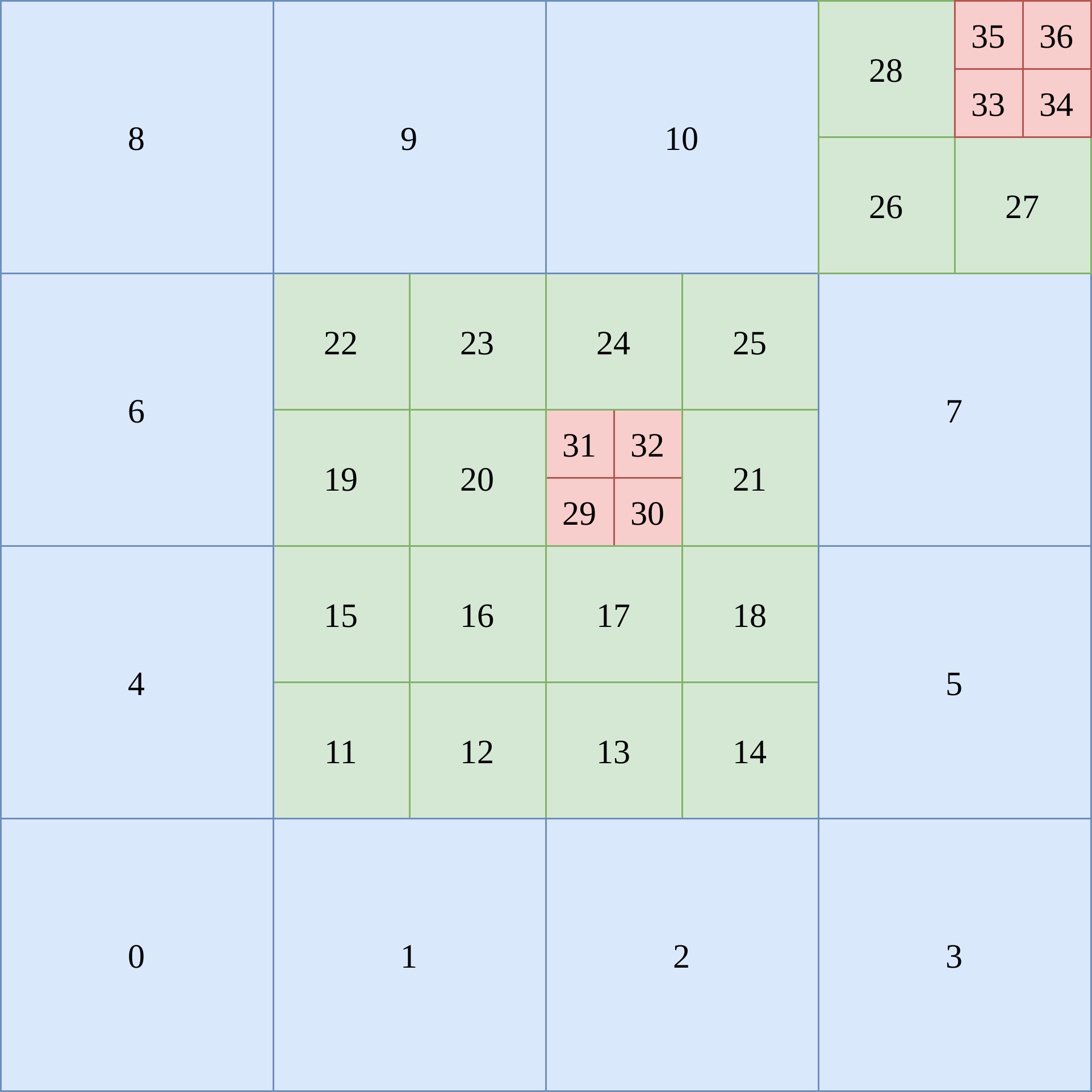
We will use the index defined by the @ operator in the intervals in the x-directions to create the link between field(level, i, j) and the cells.
For example, we have
field(0, 0, 0) is the entry 0 and pertains to the interval \([0, 4[\) for y=0,
field(2, 14, 15) is the entry 35 and pertains to the interval \([14, 16[\) for y=15.
Using the @index, we want to find the entry from the interval. The interval \([14, 16[\) for y=15 at level 2 is connected to the entries \([35, 36]\) in the field array. Therefore, if we choose the @index equal to 21 we can easily find the entries in the field array from the interval in the x-direction.
The whole samurai::CellArray is given by
level 0:
    x: [0, 4[@0, [0, 1[@4, [3, 4[@2, [0, 1[@6, [3, 4[@4, [0, 3[@8
    y: [0, 4[@0
    y-offset: [0, 1, 3, 5, 6]

level 1:
    x: [2, 6[@9, [2, 6[@13, [2, 4[@17, [5, 6[@16, [2, 6[@20, [6, 8[@20, [6, 7[@22
    y: [2, 8[@-2
    y-offset: [0, 1, 3, 5, 6, 7, 8]

level 2:
    x: [8, 10[@21, [8, 10[@23, [14, 16[@19, [14, 16[@21
    y: [8, 10[@-8, [14, 16[@-12
    y-offset: [0, 1, 2, 3, 4]
The construction of a field#
The construction of a field is made using a samurai::CellArray or a derived class from samurai::Mesh.
samurai::Mesh is used to describe grids with several samurai::CellArray and offers useful methods such as :cpp_code::operator[], :cpp_code::nb_cells, …
We shall describe more precisely how to use it in a next tutorial.
The example below shows how to initialize a vectorial field of type double with 2 components, over a mesh mesh.
auto u = samurai::make_field<double, 2>("field_name", mesh);
The name of the field is used when we want to store the solution in HDF5 format.
The field access#
In samurai, there are several ways to access a given field.
The first one is to use a samurai::Cell together with the [] operator, as in this example
samurai::Cell<coord_index_t, dim> cell{level, indices, index};

u[cell] = ...;
samurai::Cell is defined by the level, the integer coordinates of the cell and the index where we can find this cell into the field.
For more information see the dedicated part in the first tutorial (Cell properties).
Generally, we do not have to create a cell using the constructor of samurai::Cell<coord_index_t, dim>.
We can use algorithms that perform a loop over the cells of the mesh as we will see in the next tutorial (Algorithm).
The second way is to access the elements of the field as if we were on a cartesian grid. Let us give an example to better understand how it works
u(level, i, j) = ...
If we forget the level attribute for a moment, we observe that we can access the data of the field by using the indices i, j, k as we would do on a code for a uniform structured mesh.
Here, the level is needed to know where the indices live: i=1 at level 0 is completely different from i=1 at level 10.
The other difference is that the parameter i is not a scalar but an interval.
Contrarily, the other indices (j, k, …) are scalars.
Therefore, u(level, i, j) is an array of the size of the interval i.
The operation u(level, i, j) returns a xtensor view of the field where the values for the interval i in the x-direction, j in the y-direction at level are stored. It means that we can use lazy expressions (evaluated eventually in time) as in xtensor to update the data. The library xtensor offers an API very close to NumPy as described here: From numpy to xtensor.
For example
double dx = mesh.cell_length(level);
auto x = dx * xt::arange(i.start, i.end);
auto y = dx * j;
u(level, i, j) = xt::cos(x)*xt::sin(y);
where x is a vector of the size of the interval and y is a scalar. Remember that the field u has two components, thus if they are left unspecified, this expression is applied to them both.
If we want to apply this expression only to one component, we can add a parameter at the beginning to specify which one we want to modify
u(1, level, i, j) = xt::cos(x)*xt::sin(y);
Here, we have modified the second component.